matlab - matlab中具有季节分量的最小二乘法

Question

我正在阅读一篇论文，该论文研究了过去 20 年左右每月风速数据的趋势。这篇论文使用了许多不同的统计方法，我试图在这里复制这些方法。

使用的第一种方法是以下形式的简单线性回归模型

$$ y(t) = a_{1}t + b_{1} $$

其中 $a_{1}$ 和 $b_{1}$ 可以通过标准最小二乘法确定。

然后，他们指定可以通过拟合以下形式的模型来考虑季节性信号，从而明确消除线性回归模型中的一些潜在误差:

$$ y(t) = a_{2}t + b_{2}\sin\left(\frac{2\pi}{12t} + c_{2}\right) + d_{2}$$

其中系数$a_{2}$、$b_{2}$、$c_{2}$和$d_{2}$可以通过最小二乘法确定。然后他们继续指出，该模型还使用 3、4 和 6 个月的附加谐波分量进行了测试。

以以下数据为例:

 %   1949 1950 1951 1952 1953 1954 1955 1956 1957 1958 1959 1960
y = [112  115  145  171  196  204  242  284  315  340  360  417    % Jan
     118  126  150  180  196  188  233  277  301  318  342  391    % Feb
     132  141  178  193  236  235  267  317  356  362  406  419    % Mar
     129  135  163  181  235  227  269  313  348  348  396  461    % Apr
     121  125  172  183  229  234  270  318  355  363  420  472    % May
     135  149  178  218  243  264  315  374  422  435  472  535    % Jun
     148  170  199  230  264  302  364  413  465  491  548  622    % Jul
     148  170  199  242  272  293  347  405  467  505  559  606    % Aug
     136  158  184  209  237  259  312  355  404  404  463  508    % Sep
     119  133  162  191  211  229  274  306  347  359  407  461    % Oct
     104  114  146  172  180  203  237  271  305  310  362  390    % Nov
     118  140  166  194  201  229  278  306  336  337  405  432 ]; % Dec

time = datestr(datenum(yr(:),mo(:),1));
jday = datenum(time,'dd-mmm-yyyy');
y2 = reshape(y,[],1);

plot(jday,y2)

谁能演示一下上面的模型如何用 matlab 编写？

Answer 1

请注意，您的模型实际上是线性的，我们可以使用 trigonometric identity来表明这一点。要使用非线性模型，请使用 nlinfit .

使用您的数据，我编写了以下脚本来计算和比较不同的方法:

(您可以注释掉 opts.RobustWgtFun = 'bisquare'; 行，看看它与 12 周期的线性拟合完全相同)

% y = [112  115 ...
y2 = reshape(y,[],1);
t=(1:144).';

% trend
T = [ones(size(t)) t];
B=T\y2;
y_trend = T*B;

% least squeare, using linear fit and the 12 periodicity only
T = [ones(size(t)) t sin(2*pi*t/12) cos(2*pi*t/12)];
B=T\y2;
y_sincos = T*B;

% least squeare, using linear fit and 3,4,6,12 periodicities
addharmonics = [3 4 6];
T = [T bsxfun(@(h,t)sin(2*pi*t/h),addharmonics,t) bsxfun(@(h,t)cos(2*pi*t/h),addharmonics,t)];
B=T\y2;
y_sincos2 = T*B;

% least squeare with bisquare weights, 
% using non-linear model of a linear fit and the 12 periodicity only
opts = statset('nlinfit');
opts.RobustWgtFun = 'bisquare';
b0 = [1;1;0;1];
modelfun = @(b,x) b(1)*x+b(2)*sin((b(3)+x)*2*pi/12)+b(4);
b = nlinfit(t,y2,modelfun,b0,opts);

% plot a comparison
figure
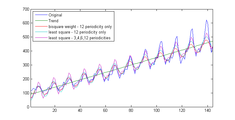
plot(t,y2,t,y_trend,t,modelfun(b,t),t,y_sincos,t,y_sincos2)
legend('Original','Trend','bisquare weight - 12 periodicity only', ...
    'least square - 12 periodicity only','least square - 3,4,6,12 periodicities', ...
    'Location','NorthWest');
xlim(minmax(t'));