我有一个准二项式 glm,其中有两个连续解释变量(假设“LogPesticide”和“LogFood”)和一个交互作用。我想计算不同食物量(例如最小和最大食物值)下农药的 LC50 和置信区间。如何实现这一目标?
示例:首先我生成一个数据集。
mydata <- data.frame(
            LogPesticide = rep(log(c(0, 0.1, 0.2, 0.4, 0.8, 1.6) + 0.05), 4),
            LogFood = rep(log(c(1, 2, 4, 8)), each = 6)
          )

set.seed(seed=16)

growth <- function(x, a = 1, K = 1, r = 1) {            # Logistic growth function. a = position of turning point
  Fx <- (K * exp(r * (x - a))) / (1 + exp(r * (x - a))) # K = carrying capacity
  return(Fx)                                            # r = growth rate (larger r -> narrower curve)
}

y <- rep(NA, length = length(mydata$LogPesticide))
y[mydata$LogFood == log(1)] <- growth(x = mydata$LogPesticide[mydata$LogFood == log(1)], a = log(0.1), K = 1, r = 6)
y[mydata$LogFood == log(2)] <- growth(x = mydata$LogPesticide[mydata$LogFood == log(2)], a = log(0.2), K = 1, r = 4)
y[mydata$LogFood == log(4)] <- growth(x = mydata$LogPesticide[mydata$LogFood == log(4)], a = log(0.4), K = 1, r = 3)
y[mydata$LogFood == log(8)] <- growth(x = mydata$LogPesticide[mydata$LogFood == log(8)], a = log(0.8), K = 1, r = 1)
mydata$Dead <- rbinom(n = length(y), size = 20, prob = y)
mydata$Alive <- 20 - mydata$Dead
mydata$Mortality <- cbind(mydata$Dead, mydata$Alive)
然后我就适应了完整的glm。模型诊断正常,所有交互项都很重要。
model <- glm(Mortality ~ LogPesticide * LogFood, family = quasibinomial, data = mydata)
plot(model)
Anova(model)
summary(model)
我尝试使用 MASS 包中的ose.p() 来估计 LC50。如果 LogFood 是一个因素,那么当我按照 this post 中讨论的那样重新拟合模型时,这将起作用。 。但对于两个连续的解释变量,您只能得到 1 个截距、2 个斜率和一个斜率差(对于交互作用)。
我可以使用effect()估计LC50,但不知道如何获取LogPesticide的相关CI。
# Create a set of fitted values.

library(effects)

food.min <- round(min(model$model$LogFood), 3)
food.max <- round(max(model$model$LogFood), 3)

eff <- effect("LogPesticide:LogFood", model,
              xlevels = list(LogPesticide = seq(min(model$model$LogPesticide), max(model$model$LogPesticide), length = 100),
                             LogFood = c(food.min, food.max)))

eff2 <- as.data.frame(eff)


# Find fitted values closest to 0.5 when LogFood is minimal and maximal.

fit.min <- which.min(abs(eff2$fit[eff2$LogFood == food.min] - 0.5))
fit.min <- eff2$fit[eff2$LogFood == food.min][fit.min]

fit.max <- which.min(abs(eff2$fit[eff2$LogFood == food.max] - 0.5))
fit.max <- eff2$fit[eff2$LogFood == food.max][fit.max]


# Use those fitted values to predict the LC50s.

lc50.min <- eff2$LogPesticide[eff2$fit == fit.min & eff2$LogFood == food.min]
lc50.max <- eff2$LogPesticide[eff2$fit == fit.max & eff2$LogFood == food.max]


# Plot the results.

plot(fit ~ LogPesticide, data = eff2[eff2$LogFood == round(min(model$model$LogFood), 3),], type = "l")
lines(fit ~ LogPesticide, data = eff2[eff2$LogFood == round(max(model$model$LogFood), 3),], col = "red")
points(y = 0.5, x = lc50.min, pch = 19)
points(y = 0.5, x = lc50.max, pch = 19, col = "red")
从dose.p()的代码中我看到必须使用vcov矩阵。 effect() 还提供了 vcov 矩阵,但我无法修改dose.p() 来正确使用该信息。如果有任何想法,我将不胜感激!
最佳答案
复制数据(更新:新版本的ggplot2可能不喜欢其中包含矩阵的奇怪数据框??)
mydata <- data.frame(
        LogPesticide = rep(log(c(0, 0.1, 0.2, 0.4, 0.8, 1.6) + 0.05), 4),
        LogFood = rep(log(c(1, 2, 4, 8)), each = 6)
      )
set.seed(seed=16)

growth <- function(x, a = 1, K = 1, r = 1) {
    ## Logistic growth function. a = position of turning point
    ## K = carrying capacity
    ## r = growth rate (larger r -> narrower curve)
    return((K * exp(r * (x - a))) / (1 + exp(r * (x - a))))
}

rlf <- data.frame(LogFood=log(c(1,2,4,8)),
                              a=log(c(0.1,0.2,0.4,0.8)),
                              r=6,4,3,1)
mydata <- merge(mydata,rlf)
mydata <- plyr::mutate(mydata,
               y=growth(LogPesticide,a,K=1,r),
               Dead=rbinom(n=nrow(mydata),size=20,prob=y),
               N=20,
               Alive=N-Dead,
               pmort=Dead/N)


model <- glm(pmort ~ LogPesticide * LogFood, family = quasibinomial,
          data = mydata, weights=N)
为了方便:
cc <- setNames(coef(model),c("b_int","b_P","b_F","b_PF"))
vv <- vcov(model)
dimnames(vv) <- list(names(cc),names(cc))
基本预测数据框:
pframe <- with(mydata,
         expand.grid(LogPesticide=seq(min(LogPesticide),max(LogPesticide),
                      length=51),
                     LogFood=unique(LogFood)))
pframe$pmort <- predict(model,newdata=pframe,type="response")
现在让我们来分解一下。 (log) 食品 F 和 (log) 农药 P 给定水平的预测值为
logit(surv) = b_int + b_P*P + b_F*F + b_PF*F*P
因此,F 水平上农药的 Logistic 曲线为
logit(surv) = (b_int+b_F*F) + (b_P+b_PF*F)*P
我们想知道 logit(surv) 为 0(LC50)时 P 的值,因此我们需要
0 = (b_int+b_F*F) + (b_P+b_PF*F)*P50
P50 = -(b_int+b_F*F)/(b_P+b_PF*F)
转换为代码:
P50mean <- function(logF) {
    with(as.list(cc), -(b_int+b_F*logF)/(b_P+b_PF*logF))
}
with(mydata,P50mean(c(min=min(LogFood),max=max(LogFood))))


pLC50 <- data.frame(LogFood=unique(mydata$LogFood))
pLC50 <- transform(pLC50,
               pmort=0.5,
               LogPesticide=P50mean(LogFood))
要获得置信区间,两种最简单的方法是 (1) delta 方法和 (2) 后验预测区间(在某些情况下也称为“参数贝叶斯”)。 (您也可以进行非参数引导。)
Delta 方法
我尝试手动完成此操作,但意识到它变得太复杂了(所有四个系数都强相关,并且必须在计算中跟踪所有这些相关性 - 这并不像通常的公式那么容易分子和分母是独立的值...)
library("emdbook")
deltavar(-(b_int+b_F*2)/(b_P+b_PF*2),meanval=cc,Sigma=vv)
## have to be a bit fancy here with eval/substitute ...
pLC50$var1 <- sapply(pLC50$LogFood,
            function(logF)
                 eval(substitute(
                     deltavar(-(b_int+b_F*logF)/(b_P+b_PF*logF),
                               meanval=cc,Sigma=vv),
                     list(logF=logF))))
总体预测区间
这假设(稍微弱一些)参数的采样分布是多元正态分布。
PP <- function(logF,n=1000) {
    b <- MASS::mvrnorm(n,mu=cc,Sigma=vv)
    pred <- with(as.data.frame(b),
         -(b_int+b_F*logF)/(b_P+b_PF*logF))
    return(var(pred))
}
set.seed(101)
pLC50$var2 <- sapply(pLC50$LogFood,PP)
通过获取预测 LC50 分布的分位数,PPI 实际上可以让我们稍微放松假设……事实证明(见下文)基于 PPI 的置信区间比 Delta 稍宽一些方法,但它们相差并不远。
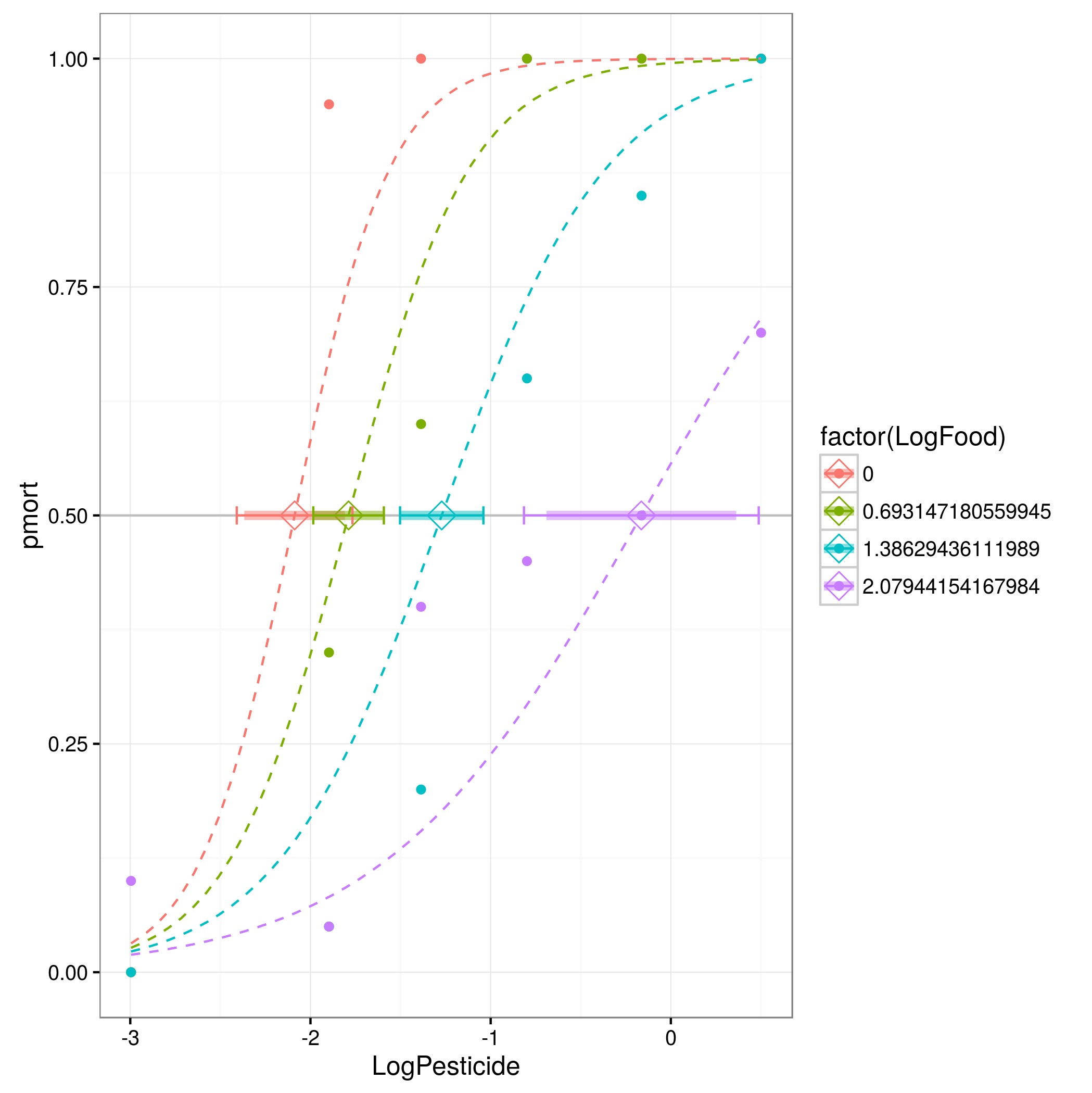
现在绘制整个困惑的情况:
library(ggplot2); theme_set(theme_bw())
gg0 <- ggplot(mydata,aes(LogPesticide,pmort,
              colour=factor(LogFood),
              fill = factor(LogFood))) + geom_point() +
       ## individual fits -- a bit ugly
       ##       geom_smooth(method="glm",aes(weight=N),
       ##           method.args=list(family=binomial),alpha=0.1)+
       geom_line(data=pframe,linetype=2)+
       geom_point(data=pLC50,pch=5,size=4)+
       geom_hline(yintercept=0.5,col="gray")

 gg0 + geom_errorbarh(data=pLC50,lwd=2,alpha=0.5,
                       aes(xmin=LogPesticide-1.96*sqrt(var1),
                           xmax=LogPesticide+1.96*sqrt(var1)),
                       height=0)+
       geom_errorbarh(data=pLC50,
                       aes(xmin=LogPesticide-1.96*sqrt(var2),
                           xmax=LogPesticide+1.96*sqrt(var2)),
                      height=0.02)
关于r - 来自具有交互作用的多元回归 glm 的 LC50/LD50 置信区间,我们在Stack Overflow上找到一个类似的问题: https://stackoverflow.com/questions/35462144/