python - 如何强制零截距来拟合二阶函数？ (Python)

Question

我正在尝试拟合具有零截距的二阶函数。现在，当我绘制它时，我得到一条 y-int > 0 的线。我试图适应该函数输出的一组点:

y**2 = 14.29566 * np.pi * x

或

y = np.sqrt(14.29566 * np.pi * x)

两个数据集 x 和 y，其中 D = 3.57391553。我的试衣习惯是:

z = np.polyfit(x,y,2)                         # Generate curve coefficients
p = np.poly1d(z)                              # Generate curve function

xp = np.linspace(0, catalog.tlimit, 10)       # generate input values

plt.scatter(x,y)
plt.plot(xp, p(xp), '-')
plt.show()

我也尝试过使用statsmodels.ols:

mod_ols = sm.OLS(y,x)
res_ols = mod_ols.fit()

但我不明白如何为二阶函数(而不是线性函数)生成系数，也不明白如何将 y-int 设置为 0。我看到另一篇类似的文章涉及强制 y-int 为 0具有线性拟合，但我无法弄清楚如何使用二阶函数来做到这一点。

现在的剧情:

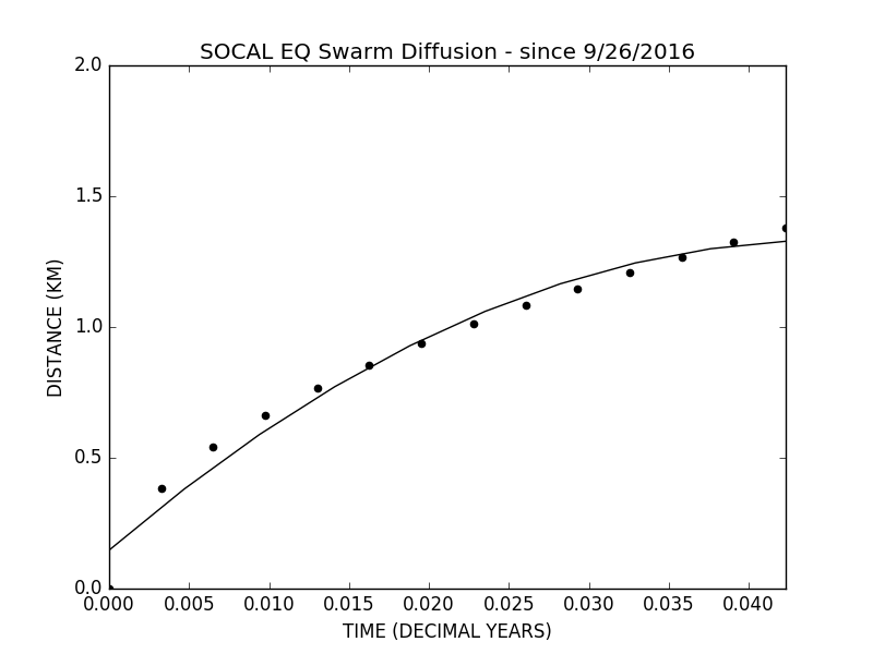
数据:

x = [0., 0.00325492, 0.00650985, 0.00976477, 0.01301969, 0.01627462, 0.01952954, 0.02278447, 
     0.02603939, 0.02929431, 0.03254924, 0.03580416, 0.03905908, 0.04231401]
y = [0., 0.38233801, 0.5407076, 0.66222886, 0.76467602, 0.85493378, 0.93653303, 1.01157129,
     1.0814152, 1.14701403, 1.20905895, 1.26807172, 1.32445772, 1.3785393]

Answer 1

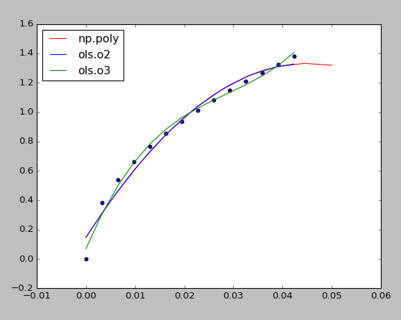
如果我理解正确，您想用OLS拟合多项式回归线，您可以尝试以下操作(正如我们所见，随着拟合多项式的次数增加，模型会过度拟合数据越来越多):

xp = np.linspace(0, 0.05, 10)       # generate input values
pred1 = p(xp)  # prediction with np.poly as you have done

import pandas as pd
data = pd.DataFrame(data={'x':x, 'y':y})

# let's first fit 2nd order polynomial with OLS with intercept
olsres2 = sm.ols(formula = 'y ~ x + I(x**2)', data = data).fit()
print olsres2.summary()


                             OLS Regression Results
==============================================================================
Dep. Variable:                      y   R-squared:                       0.978
Model:                            OLS   Adj. R-squared:                  0.974
Method:                 Least Squares   F-statistic:                     243.1
Date:                Sat, 21 Jan 2017   Prob (F-statistic):           7.89e-10
Time:                        04:16:22   Log-Likelihood:                 20.323
No. Observations:                  14   AIC:                            -34.65
Df Residuals:                      11   BIC:                            -32.73
Df Model:                           2
Covariance Type:            nonrobust
==============================================================================
                 coef    std err          t      P>|t|      [95.0% Conf. Int.]
------------------------------------------------------------------------------
Intercept      0.1470      0.045      3.287      0.007         0.049     0.245
x             52.4655      4.907     10.691      0.000        41.664    63.267
I(x ** 2)   -580.4730    111.820     -5.191      0.000      -826.588  -334.358
==============================================================================
Omnibus:                        4.803   Durbin-Watson:                   1.164
Prob(Omnibus):                  0.091   Jarque-Bera (JB):                2.101
Skew:                          -0.854   Prob(JB):                        0.350
Kurtosis:                       3.826   Cond. No.                     6.55e+03
==============================================================================

pred2 = olsres2.predict(data) # predict with the fitted model
# fit 3rd order polynomial with OLS with intercept
olsres3 = sm.ols(formula = 'y ~ x + I(x**2) + I(x**3)', data = data).fit()
pred3 = olsres3.predict(data) # predict

plt.scatter(x,y)
plt.plot(xp, pred1, '-r', label='np.poly')
plt.plot(x, pred2, '-b', label='ols.o2')
plt.plot(x, pred3, '-g', label='ols.o3')
plt.legend(loc='upper left')
plt.show()

# now let's fit the polynomial regression lines this time without intercept
olsres2 = sm.ols(formula = 'y ~ x + I(x**2)-1', data = data).fit()
print olsres2.summary()
                                OLS Regression Results
==============================================================================
Dep. Variable:                      y   R-squared:                       0.993
Model:                            OLS   Adj. R-squared:                  0.992
Method:                 Least Squares   F-statistic:                     889.6
Date:                Sat, 21 Jan 2017   Prob (F-statistic):           9.04e-14
Time:                        04:16:24   Log-Likelihood:                 15.532
No. Observations:                  14   AIC:                            -27.06
Df Residuals:                      12   BIC:                            -25.79
Df Model:                           2
Covariance Type:            nonrobust
==============================================================================
                 coef    std err          t      P>|t|      [95.0% Conf. Int.]
------------------------------------------------------------------------------
x             65.8170      3.714     17.723      0.000        57.726    73.908
I(x ** 2)   -833.6787    109.279     -7.629      0.000     -1071.777  -595.580
==============================================================================
Omnibus:                        1.716   Durbin-Watson:                   0.537
Prob(Omnibus):                  0.424   Jarque-Bera (JB):                1.341
Skew:                           0.649   Prob(JB):                        0.511
Kurtosis:                       2.217   Cond. No.                         118.
==============================================================================
pred2 = olsres2.predict(data)
# fit 3rd order polynomial with OLS without intercept
olsres3 = sm.ols(formula = 'y ~ x + I(x**2) + I(x**3) -1', data = data).fit()
pred3 = olsres3.predict(data)

plt.scatter(x,y)
plt.plot(xp, pred1, '-r', label='np.poly')
plt.plot(x, pred2, '-b', label='ols.o2')
plt.plot(x, pred3, '-g', label='ols.o3')
plt.legend(loc='upper left')
plt.show()