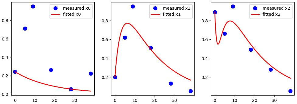
给定数据x0、x1和x2,假设我想要拟合参数k0、以下 ODE 系统中的 k1、k2、p1 和 p2
下面的代码可以实现我想要的功能
pip install lmfit
import numpy as np
import matplotlib.pyplot as plt
from scipy.integrate import odeint
from lmfit import minimize, Parameters, report_fit

# Function definitions
def f(y, t, paras):
    """
    System of differential equations
    """

    x0 = y[0]
    x1 = y[1]
    x2 = y[2]

    try:
        k0 = paras['k0'].value
        k1 = paras['k1'].value
        k2 = paras['k2'].value
        p1 = paras['p1'].value
        p2 = paras['p2'].value
    except KeyError:
        k0, k1, k2, p1, p2 = paras

    # Updated model equations
    f0 = -k0 * x0
    f1 = p1 * x0 - k1 * x1
    f2 = p2 * x1 - k2 * x2
    return [f0, f1, f2]

def g(t, x000, paras):
    """
    Solution to the ODE x'(t) = f(t,x,k) with initial condition x(0) = x000
    """
    x = odeint(f, x000, t, args=(paras,))
    return x

def residual(paras, t, data):
    x000 = paras['x00'].value, paras['x10'].value, paras['x20'].value
    model = g(t, x000, paras)

    # Assume you have data for x1 and x3 as well
    x0_model = model[:, 0]
    x1_model = model[:, 1]
    x2_model = model[:, 2]

    # Compute residuals for all variables
    return np.concatenate([(x0_model - data['x0']).ravel(),
                           (x1_model - data['x1']).ravel(),
                           (x2_model - data['x2']).ravel()])


# Measured data
t_measured = np.array([0, 5, 9, 18, 28, 38])
x0_measured = np.array([0.24, 0.71, 0.95, 0.26, 0.05, 0.22])
x1_measured = np.array([0.2, 0.62, 0.95, 0.51, 0.13, 0.05])
x2_measured = np.array([0.89, 0.66, 0.95, 0.49, 0.28, 0.05])

# Initial conditions
x00 = x0_measured[0]
x10 = x1_measured[0]
x20 = x2_measured[0]
y0 = [x00, x10, x20]

# Data dictionary
data = {'x0': x0_measured, 'x1': x1_measured, 'x2': x2_measured}

# Set parameters including bounds
params = Parameters()
params.add('x00', value=x00, vary=False)
params.add('x10', value=x10, vary=False)
params.add('x20', value=x20, vary=False)
params.add('k0', value=0.2, min=0.0001, max=2.)
params.add('k1', value=0.3, min=0.0001, max=2.)
params.add('k2', value=0.1, min=0.0001, max=2.)  # Assuming k2 is needed
params.add('p1', value=0.1, min=0.0001, max=2.)  # Assuming p1 is needed
params.add('p2', value=0.1, min=0.0001, max=2.)  # Assuming p2 is needed

# Fit model
result = minimize(residual, params, args=(t_measured, data), method='leastsq')  # leastsq nelder
# Check results of the fit
data_fitted = g(np.linspace(0., 38., 100), y0, result.params)

# Updated plotting to include x0, x1, and x2
plt.figure(figsize=(12, 4))

plt.subplot(1, 3, 1)
plt.scatter(t_measured, x0_measured, marker='o', color='b', label='measured x0', s=75)
plt.plot(np.linspace(0., 38., 100), data_fitted[:, 0], '-', linewidth=2, color='red', label='fitted x0')
plt.legend()

plt.subplot(1, 3, 2)
plt.scatter(t_measured, x1_measured, marker='o', color='b', label='measured x1', s=75)
plt.plot(np.linspace(0., 38., 100), data_fitted[:, 1], '-', linewidth=2, color='red', label='fitted x1')
plt.legend()

plt.subplot(1, 3, 3)
plt.scatter(t_measured, x2_measured, marker='o', color='b', label='measured x2', s=75)
plt.plot(np.linspace(0., 38., 100), data_fitted[:, 2], '-', linewidth=2, color='red', label='fitted x2')
plt.legend()

plt.show()
现在,我不想用 ODE 来拟合 x0,而是想对其进行插值,这样我就有更多的自由。理想情况下,我想定义一个(或多个)插值参数,该参数也将进入优化问题。关于最好的方法有什么想法吗?
我的想法:类似于this answer in Mathematica ,我们可以考虑一个定制的插值函数,该函数将为连续数据点之间的每个间隔获取一个参数,该参数将全部与其余参数 k1、k2 进行拟合。 ,原系统中的p1和p2。我不确定这是否理想(或快速),但如果我们忽略 x0 的第一个方程并使用插值代替,它会给出更好的近似值。例如,使用以下插值的参数化版本
from scipy.interpolate import UnivariateSpline
spline = UnivariateSpline(t_measured, x0_measured)
x0_spline = spline(t_interpolated)
plt.figure(figsize=(8, 4))
plt.scatter(t_measured, x0_measured, color='blue', label='Measured x0', zorder=3)
plt.plot(t_interpolated, x0_spline, color='green', linestyle='-', label='Spline Interpolation of x0')
plt.title("Spline Interpolation of x0")
plt.xlabel("Time")
plt.ylabel("x0")
plt.legend()
plt.grid(True)
plt.show()

最佳答案
如果您的数据集可以通过您的模型进行拟合,则它可能会错过观测值 ( curse of dimensionality )。
您的程序可能是正确的,但由于缺少点而无法正确收敛。拥有 3x6 点似乎不足以为这个具有 5 个未知参数的 3D ODE 系统塑造适当的误差景观。
这是一个无需插值即可执行优化的过程(委托(delegate)给 solve_ivp)来与结果进行交叉检查:
import numpy as np
import matplotlib.pyplot as plt
from scipy import integrate, optimize

def system(t, x, k0, k1, k2, p1, p2):
    return np.array([
        -k0 * x[0],
        p1 * x[0] - k1 * x[1],
        p2 * x[1] - k2 * x[2]
    ])

def solver(parameters, t=np.linspace(0, 1, 10), x0=np.ones(3)):
    solution = integrate.solve_ivp(system, [t.min(), t.max()], x0, args=parameters, t_eval=t)
    return solution.y

def residuals_factory(t, x):
    def wrapped(parameters):
        return 0.5 * np.sum(np.power(x - solver(parameters, t=t, x0=x[:, 0]), 2))
    return wrapped


# Synthetic dataset:
texp = np.linspace(0, 35, 15)
p0 = np.array([ 0.03693555,  0.38054633, -0.06252069,  1.41453107, -0.11159681])
x0 = np.array([0.24, 0.20, 0.89])
xexp = solver(p0, t=texp, x0=x0)

# Optimization
residuals = residuals_factory(texp, xexp)
solution = optimize.minimize(residuals, x0=[1, 1, 1, 1, 1])  # Initial guess

# Regression:
tlin = np.linspace(texp.min(), texp.max(), 200)
xhat = solver(solution.x, t=tlin, x0=x0)

fig, axe = plt.subplots()
for i in range(xexp.shape[0]):
    axe.scatter(texp, xexp[i, :])
    axe.plot(tlin, xhat[i, :])
axe.grid()
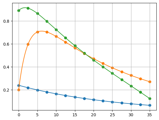
该方法能够回归初始参数,并确保拟合函数将通过初始点。如果维度少于 10 个点,收敛会更加困难。
误差景观似乎有多个最小值,这可能需要调整初始参数才能找到搜索到的最佳值。另请注意,误差函数(残差)需要足够的项和适当的噪声,以便在最佳值附近有足够的曲率和陡度来驱动梯度下降。
更新
我们可以修改回归过程来放宽通过初始点的约束。新签名如下所示:
def solver(parameters, t=np.linspace(0, 1, 10)):
    x0 = parameters[-3:]
    parameters = parameters[:-3]
    solution = integrate.solve_ivp(system, [t.min(), t.max()], x0, args=parameters, t_eval=t)
    return solution.y

def residuals_factory(t, x):
    def wrapped(parameters):
        return 0.5 * np.sum(np.power(x - solver(parameters, t=t), 2))
    return wrapped
那么问题有 8 个参数,因为初始条件也有影响。我们还可以将梯度下降限制为仅正常数。
residuals = residuals_factory(texp, xexp)
solution = optimize.minimize(
    residuals, x0=[1, 1, 1, 1, 1, 1, 1, 1, 1],
    bounds=[(0, np.inf)]*8
)
# array([0.05157739, 0.32032917, 0.8680015 , 0.49081592, 0.90863933, 0.68856984, 0.17679386, 0.8890076 ])
下图显示了您的数据集的结果。
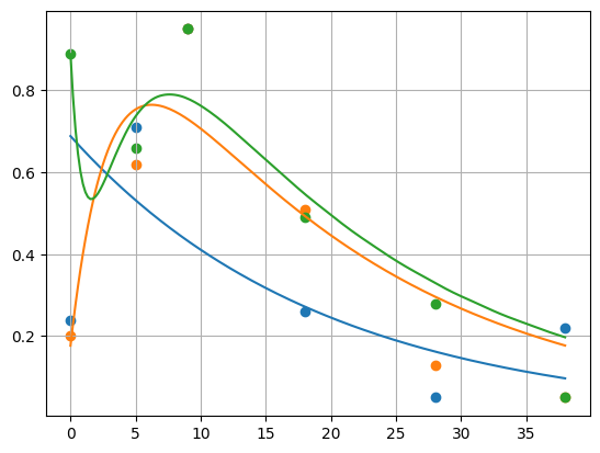
它没有太多的适应性,但它确认约束已经放松,并且允许捕获比第一个签名更多的方差。
另一方面,拟合过程仍然适用于合成数据集(已知服从模型的数据集)上具有合理噪声的 8 个参数。

观察结果
- 您的数据表现出一些模型无法拟合的振荡(例如:指数衰减仅无法拟合
x0动态); - 如果振荡是由噪声引起的,那么其幅度就很大,再加上缺乏数据(很少的点),就会导致拟合变得困难
- 可以证明,只要有足够的点和合理的数据噪声,程序就可以回归参数
你有几个选择:
- 以更高的精度为每条曲线收集更多的点(或拒绝已知为异常值的点)。这将允许您接受或拒绝当前模型;
- 如果数据点很少,请更改 ODE 模型以捕获动态,而不会增加太多复杂性(那么我们可能需要更深入地了解生成这些数据的底层流程);
- 重新表述您的问题,您是否在寻找:
- 回归:需要从模型中获取常量;
- 或插值:您想通过点(无论底层模型如何)来预测其他地方的点?
更新2
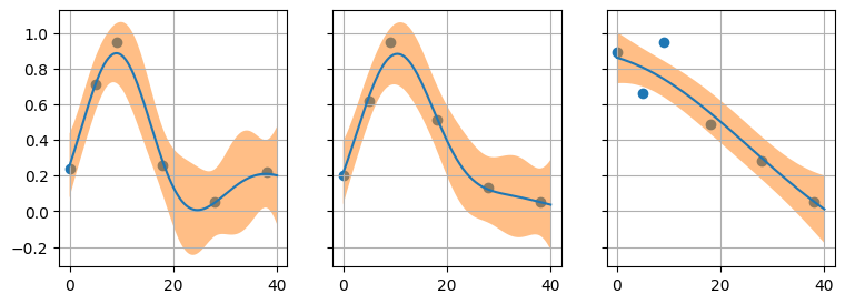
带有 RBF 内核的高斯过程可以以明显的适应性通过您的级数:
import numpy as np
import matplotlib.pyplot as plt
from sklearn.gaussian_process.kernels import RBF
from sklearn.gaussian_process import GaussianProcessRegressor

texp = np.array([0, 5, 9, 18, 28, 38]).reshape(-1, 1)
xexp = np.array([
    [0.24, 0.71, 0.95, 0.26, 0.05, 0.22],
    [0.2, 0.62, 0.95, 0.51, 0.13, 0.05],
    [0.89, 0.66, 0.95, 0.49, 0.28, 0.05]
])

tlin = np.linspace(0, 40, 200).reshape(-1, 1)
fig, axes = plt.subplots(1, 3, sharex=True, sharey=True, figsize=(9,3))

for i in range(3):

    kernel = 1 * RBF(length_scale=1.0)
    model = GaussianProcessRegressor(kernel=kernel, alpha=0.01**2)

    model.fit(texp, xexp[i, :])
    xpred, xstd = model.predict(tlin, return_std=True)

    axe = axes[i]
    axe.scatter(texp, xexp[i, :])
    axe.plot(tlin, xpred)
    axe.fill_between(tlin.ravel(), xpred - 1.96 * xstd, xpred + 1.96 * xstd, alpha=0.5)
    axe.grid()
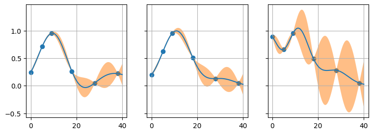
在这种情况下,您可以使用精度提示在已知数据之间预测/插值点,但没有要提取的回归参数。
您可以调整高斯过程 alpha 参数以平滑曲线(低于 alpha=0.1**2):
关于python - 如何用插值拟合 ODE 系统?,我们在Stack Overflow上找到一个类似的问题: https://stackoverflow.com/questions/77587951/