ggplot2 - 如何绘制 glm 模型(gamma 系列)的置信区间？

Question

我想从 glm 模型(系列 Gamma )中绘制直线和 95% 置信区间。对于线性模型，我以前能够根据预测绘制置信区间，因为它们包括拟合、下限和上限以及使用多边形，但我不知道如何在这里做，因为预测不包括上限和下限.我也试过 ggplot 但似乎平滑使曲线变平。在此先感谢您的帮助。见代码:

library(ggplot2)

# Data
dat <- data.frame(c(45,75,85,2,14,45,45,45,45,45,55,55,65,85,15,15,315,3,40,85,125,115,13,105,
                    145,125,145,125,205,125,155,125,19,17,145,14,85,65,135,45,40,15,14,10,15,10,10,45,37,30),
                  c(1.928607e-01, 3.038813e-01, 8.041174e-02, 0.000000e+00, 1.017541e-02, 1.658876e-01, 2.084661e-01,
                  1.891305e-01, 2.657766e-01, 1.270864e-01, 1.720141e-01, 1.644947e-01, 7.038978e-02, 3.046604e-01,
                  3.111646e-02, 9.443539e-04, 3.590906e-02, 0.000000e+00, 2.384494e-01, 5.955332e-02, 7.703567e-02,
                  5.524471e-02, 9.915716e-04, 1.169936e-01, 1.409448e-01, 1.411809e-01, 1.025096e-01, 2.649503e-01,
                  6.309465e-02, 3.727837e-02, 8.855679e-02, 1.707864e-01, 1.714002e-02, 1.038789e-03, 1.208065e-01,
                  3.541327e-04, 7.492268e-02, 9.633591e-02, 7.414359e-02, 2.235050e-01, 1.489010e-01, 2.478929e-03,
                  2.573364e-03, 5.430035e-04, 1.719905e-02, 1.243006e-02, 6.822957e-03, 1.927544e-01, 1.146918e-01, 9.030385e-03))

colnames(dat) <- c("age", "wood")  

# Model
model<- glm(wood+0.001 ~ log(age) + I(log(age)^2), data=dat, family = Gamma)
summary(model)

p<-predict(model, data.frame(age=1:200), interval="confidence", level=.95)
p.tr <- 1/p # inverse link according to ?glm

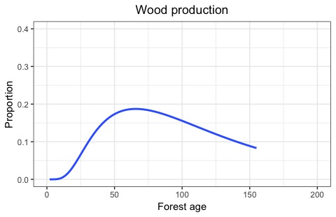
# Plot
plot(1:200, p.tr, type="n", ylim = c(0,.4), xlab="Forest age",
     ylab="Proportion",
     main="Wood production", yaxt="n")
axis(2, las=2)
lines(1:200, p.tr, ylim=range(p.tr), lwd=2, col=rgb(0, .4, 1))
# How can I add to this plot the 95% confidence intervals of the model?

# Ggplot
# I use this function because there was a warning of "Ignoring unknown parameters: family" and this solves that
binomial_smooth <- function(...) { 
  geom_smooth(method = "glm", method.args = list(family = "binomial"),formula=y~log(x)+I(log(x)^2),se=FALSE) 
} 

ggplot(dat, aes(x=age, 
                y=wood+0.001)) +
  binomial_smooth() +
  xlab("Forest age") +
  ylab("Proportion") +
  ggtitle("Wood production") +
  xlim(0, 200) +
  ylim(0,0.4) +
  theme_bw() +
  theme (plot.title = element_text(hjust = 0.5), legend.position = "none")

# Why I get this warning (Warning: In eval(family$initialize) : non-integer #successes in a binomial glm!)?
# Why is the curve more smooth here?

Answer 1

我不是数学家/统计学家，但我猜“family = binomial”给了你不恰当的估计，因为它不是正确的分布，因为 wood 和 age 都不是可数的值。

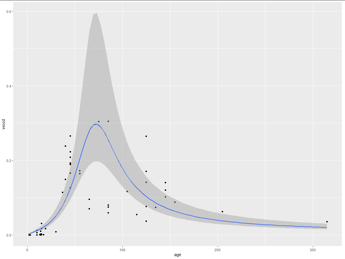
关于置信区间: 我使用了 stat_smooth()，见下文。不过应该与 geom_smooth() 相同。

dat <- data.frame(c(45,75,85,2,14,45,45,45,45,45,55,55,65,85,15,15,315,3,40,85,125,115,13,105,
                    145,125,145,125,205,125,155,125,19,17,145,14,85,65,135,45,40,15,14,10,15,10,10,45,37,30),
                  c(1.928607e-01, 3.038813e-01, 8.041174e-02, 0.000000e+00, 1.017541e-02, 1.658876e-01, 2.084661e-01,
                    1.891305e-01, 2.657766e-01, 1.270864e-01, 1.720141e-01, 1.644947e-01, 7.038978e-02, 3.046604e-01,
                    3.111646e-02, 9.443539e-04, 3.590906e-02, 0.000000e+00, 2.384494e-01, 5.955332e-02, 7.703567e-02,
                    5.524471e-02, 9.915716e-04, 1.169936e-01, 1.409448e-01, 1.411809e-01, 1.025096e-01, 2.649503e-01,
                    6.309465e-02, 3.727837e-02, 8.855679e-02, 1.707864e-01, 1.714002e-02, 1.038789e-03, 1.208065e-01,
                    3.541327e-04, 7.492268e-02, 9.633591e-02, 7.414359e-02, 2.235050e-01, 1.489010e-01, 2.478929e-03,
                    2.573364e-03, 5.430035e-04, 1.719905e-02, 1.243006e-02, 6.822957e-03, 1.927544e-01, 1.146918e-01,
                    9.030385e-03))

colnames(dat) <- c("age", "wood")

model<- glm(wood+0.001 ~ log(age) + I(log(age)^2), data=dat, family = Gamma)
#summary(model)

p<-predict(model, data.frame(age=1:200), interval="confidence", level=.95)
p.tr <- 1/p # inverse link according to ?glm

prediction <- data.frame(age = as.numeric(names(p)), wood = 1/p)


ggplot(data = dat, aes(x = age, y = wood)) +
  geom_point() +
  geom_line(data= prediction) +
  stat_smooth(data = dat, method = "glm",
              formula = y+0.001 ~ log(x) + I(log(x)^2),
              method.args = c(family = Gamma))