我知道如何在 R 中进行基本多项式回归。但是,我只能使用 nls 或 lm 来拟合一条线,以最大限度地减少点的误差。
这在大多数情况下都有效,但有时当数据中存在测量差距时,模型就会变得非常违反直觉。有没有办法添加额外的约束?
可重现的示例:
我想将模型拟合到以下虚构数据(类似于我的真实数据):
x <- c(0, 6, 21, 41, 49, 63, 166)
y <- c(3.3, 4.2, 4.4, 3.6, 4.1, 6.7, 9.8)
df <- data.frame(x, y)
首先,让我们绘制它。
library(ggplot2)
points <- ggplot(df, aes(x,y)) + geom_point(size=4, col='red')
points
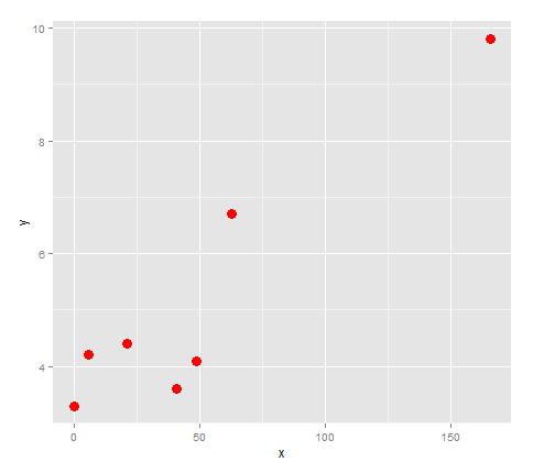
看起来如果我们用一条线连接这些点,它会改变方向 3 次,所以让我们尝试对其进行四次拟合。
lm <- lm(formula = y ~ x + I(x^2) + I(x^3) + I(x^4))
quartic <- function(x)  lm$coefficients[5]*x^4 + lm$coefficients[4]*x^3 + lm$coefficients[3]*x^2 + lm$coefficients[2]*x + lm$coefficients[1]

points + stat_function(fun=quartic)
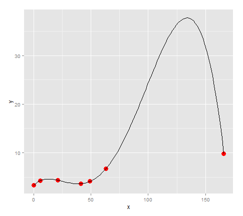
看起来模型非常适合这些点...除了,因为我们的数据在 63 和 166 之间有很大差距,所以那里有一个巨大的尖峰,没有理由出现在模型中。 (对于我的实际数据,我知道那里没有巨大的峰值)
所以本例中的问题是:
- 如何将局部最大值设置为 (166, 9.8)?
如果这是不可能的,那么另一种方法是:
- 如何限制该线预测的 y 值不大于 y=9.8。
或者也许有更好的模型可以使用? (除了分段进行之外)。我的目的是比较图之间模型的特征。
最佳答案
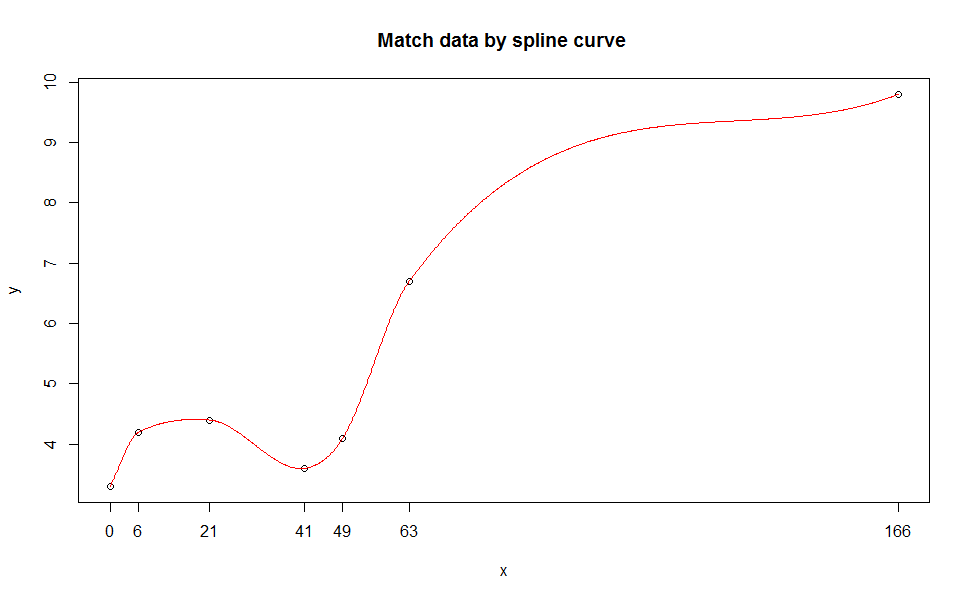
spline 类型的函数将与您的数据完美匹配(但不用于预测目的)。样条曲线广泛应用于CAD领域,有时它只是拟合数学上的数据点,与回归相比可能缺乏物理意义。更多信息here以及 here 中的精彩背景介绍.
示例(样条线)将向您展示许多奇特的示例,实际上我使用了其中一个。
此外,采样更多的数据点,然后通过lm或nls回归进行预测会更加合理。
示例代码:
library(splines)

x <- c(0, 6, 21, 41, 49, 63, 166)
y <- c(3.3, 4.2, 4.4, 3.6, 4.1, 6.7, 9.8)

s1 <- splinefun(x, y, method = "monoH.FC")

plot(x, y)
curve(s1(x), add = TRUE, col = "red", n = 1001)
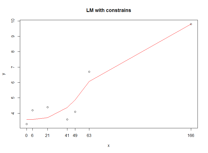
我能想到的另一种方法是在回归中限制参数范围,以便您可以获得预期范围内的预测数据。
非常简单的代码,下面有 optim,但只有一个选择。
dat <- as.data.frame(cbind(x,y))
names(dat) <- c("x", "y")

# your lm
# lm<-lm(formula = y ~ x + I(x^2) + I(x^3) + I(x^4))

# define loss function, you can change to others
 min.OLS <- function(data, par) {
      with(data, sum((   par[1]     +
                         par[2] *  x +
                         par[3] * (x^2) +
                         par[4] * (x^3) +
                         par[5] * (x^4) +
                         - y )^2)
           )
 }

 # set upper & lower bound for your regression
 result.opt <- optim(par = c(0,0,0,0,0),
                min.OLS,
                data = dat,
                lower=c(3.6,-2,-2,-2,-2),
                upper=c(6,1,1,1,1),
                method="L-BFGS-B"
  )

 predict.yy <- function(data, par) {
               print(with(data, ((
                    par[1]     +
                    par[2] *  x +
                    par[3] * (x^2) +
                    par[4] * (x^3) +
                    par[5] * (x^4))))
                )
  }

  plot(x, y, main="LM with constrains")
  lines(x, predict.yy(dat, result.opt$par), col="red" )
关于r - R 中的多项式回归 - 对曲线有额外的约束,我们在Stack Overflow上找到一个类似的问题: https://stackoverflow.com/questions/34170235/